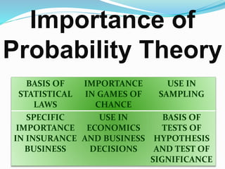
Key Takeaway: A probability distribution is a mathematical description of how likely each possible outcome of a random variable is, and it forms the foundation of actuarial pricing, financial risk modeling, quality control, and statistical inference generally. The critical distinction from an ordinary variable is that a random variable has no single fixed value until an outcome is actually observed. What is defined in advance is not a value, but the entire distribution of possible values and their associated probabilities.
Most quantitative disciplines, actuarial science, finance, engineering, and epidemiology among them, rest on a small set of mathematical tools that rarely get explained plainly. Probability distributions are the most consequential of these tools, since almost every model used to price insurance, assess financial risk, or forecast uncertain outcomes is, at its core, a choice of which distribution best represents the underlying randomness. Understanding what a distribution actually is, and how it differs from the variables most people are taught in basic algebra, is a prerequisite for evaluating whether any quantitative model deserves trust.
What a Probability Distribution Actually Is
Formally, a probability distribution specifies the probabilities associated with all possible values a random variable can take. For a discrete random variable, one that can only take a countable set of values, this is called a probability mass function, denoted P(X = x), which assigns a specific probability to each possible outcome. For a continuous random variable, one that can take any value within a range, the equivalent is a probability density function, where probabilities are found by integrating the function over an interval rather than reading a value at a single point, since the probability of any single exact value is technically zero for a continuous variable. Both discrete and continuous distributions can also be described by a cumulative distribution function, which gives the probability that the random variable takes a value less than or equal to a given number, and which applies uniformly across both variable types.
Random Variables Versus Ordinary Variables
This is the distinction most often misunderstood outside formal statistics training. An ordinary variable, the kind used in algebra or programming, holds a specific, determinate value. Writing x = 5 assigns a fixed quantity to x, and solving an equation for x is a search for that one correct value. A random variable is fundamentally different. Formally, it is a function that maps the outcomes of a random process, technically the elements of a sample space, to real numbers. Before the random process occurs, the random variable does not have a determined value. What exists instead is a complete probability distribution describing every value the variable could take and how likely each one is. Only after the random process actually occurs does the random variable take on what is called a realization, a specific observed value drawn from that distribution. Rolling a die illustrates this cleanly. Before the roll, the outcome is a random variable governed by a uniform distribution across the values one through six. After the roll, a specific number is observed, which is the realization, not the random variable itself. Conflating the two, treating a random variable as though it already holds a fixed value before observation, is one of the most common conceptual errors in applied statistics and a frequent source of miscommunication between technical and non technical stakeholders.
Common Distributions and Where Each One Is Actually Used
Different real world phenomena are better represented by different distribution shapes, and choosing the wrong one is a frequent source of model error. Among discrete distributions, the binomial distribution models the number of successes across a fixed number of independent trials with a constant probability of success, making it standard for modeling whether an insurance claim occurs at all across a block of policies. The Poisson distribution models the number of rare, independent events occurring within a fixed interval of time or space, and is the standard choice for modeling claim frequency in actuarial ratemaking, as well as applications like call center arrivals or network failure counts. Among continuous distributions, the normal or Gaussian distribution is the most widely used, both because many natural measurement processes approximate it and because of the central limit theorem, which states that the distribution of a sample mean approaches normality as sample size increases, regardless of the underlying population's distribution, provided that population has finite variance. This theorem is the mathematical reason the normal distribution appears so pervasively throughout statistical inference, even when the underlying data itself is not normally distributed. The exponential distribution models the time between independent events occurring at a constant average rate, and is standard in reliability engineering and survival analysis. The lognormal distribution, where the logarithm of the variable is normally distributed, is commonly used to model insurance claim severity and asset prices, since it naturally restricts values to be positive and captures right skewed behavior. Heavier tailed distributions such as the Pareto distribution are specifically used in catastrophe and extreme value modeling, since normal distributions systematically understate the probability of extreme, low frequency, high severity events.
Why This Matters Beyond the Mathematics
The practical value of choosing the correct distribution is best illustrated by frequency severity modeling in actuarial pricing, where claim frequency and claim severity are modeled as two separate random variables, typically a Poisson distribution for frequency and a lognormal or Pareto distribution for severity, then combined to estimate the aggregate loss distribution an insurer must price and reserve against. Using an inappropriate distribution, for instance modeling claim severity with a normal distribution when the real data is heavily right skewed, will systematically understate the probability and magnitude of large losses. This exact failure mode, underestimating tail risk by defaulting to normal distribution assumptions, has been widely identified as a contributing factor in several historical financial modeling failures, since real financial returns tend to exhibit heavier tails than a normal distribution predicts.
What This Means for Decision-Makers
Organizations relying on quantitative risk models should ask explicitly which distribution underlies any forecast, price, or reserve estimate they are given, rather than accepting a single point estimate at face value. A single number derived from a probability distribution, such as an expected loss or a mean forecast, discards information about the spread and shape of possible outcomes that often matters more than the average itself, particularly for rare but severe events. Decision makers evaluating a risk model should specifically ask whether the tails of the assumed distribution are heavy enough to reflect real world extreme events, since defaulting to a normal distribution for convenience is a documented and recurring source of underestimated risk. Where a model's underlying distributional assumptions are not disclosed or justified, that omission itself should be treated as a red flag rather than a technical detail safe to ignore.
Sources & Further Reading
- NIST/SEMATECH e-Handbook of Statistical Methods, Chapter 1: Exploratory Data Analysis — itl.nist.gov
- MIT OpenCourseWare, 18.05 Introduction to Probability and Statistics — ocw.mit.edu
- Society of Actuaries, Exam P (Probability) Syllabus and Study Materials — soa.org
- Casella, G. and Berger, R. L., Statistical Inference, 2nd Edition
- Youtube Video :https://riskbynumbers.org/
Comments